Databricks ETL Optimization for Petabyte Data

Handling petabyte-scale data in ETL pipelines requires precise tuning to prevent slowdowns, reduce costs, and maintain efficiency. This article explains how to optimize Databricks for massive datasets, addressing common challenges like data skew, shuffle operations, and the tiny files problem.

Key takeaways:

• Databricks Features: Use Photon Engine for faster joins (up to 12x), Delta Lake for reliable data storage, and serverless compute for scalability.
• Cluster Configuration: Choose the right instance types, enable autoscaling, and use spot instances to cut costs by 40-60%.
• Data Layout: Apply liquid clustering or Z-ordering for faster queries and efficient storage.
• Performance Tuning: Enable Adaptive Query Execution (AQE), adjust shuffle partitions, and monitor Spark UI metrics to resolve bottlenecks.
• File Management: Consolidate small files with OPTIMIZE and use predictive optimization for automated maintenance.

Databricks helps organizations process petabyte-scale data with reduced runtimes (up to 80% faster) and lower compute costs (up to 40%). By fine-tuning configurations, managing data storage efficiently, and leveraging advanced features, you can ensure your ETL pipelines remain scalable and cost-effective.

Stop Manual Tuning: Predictive Optimization in Databricks Explained

sbb-itb-61a6e59

Configuring Databricks Clusters for Large-Scale ETL

Getting your cluster settings right is essential for running a smooth and cost-effective petabyte-scale ETL pipeline. Databricks offers various cluster configurations and scaling options tailored for handling large workloads efficiently.

Selecting the Right Cluster Type and Instance Sizes

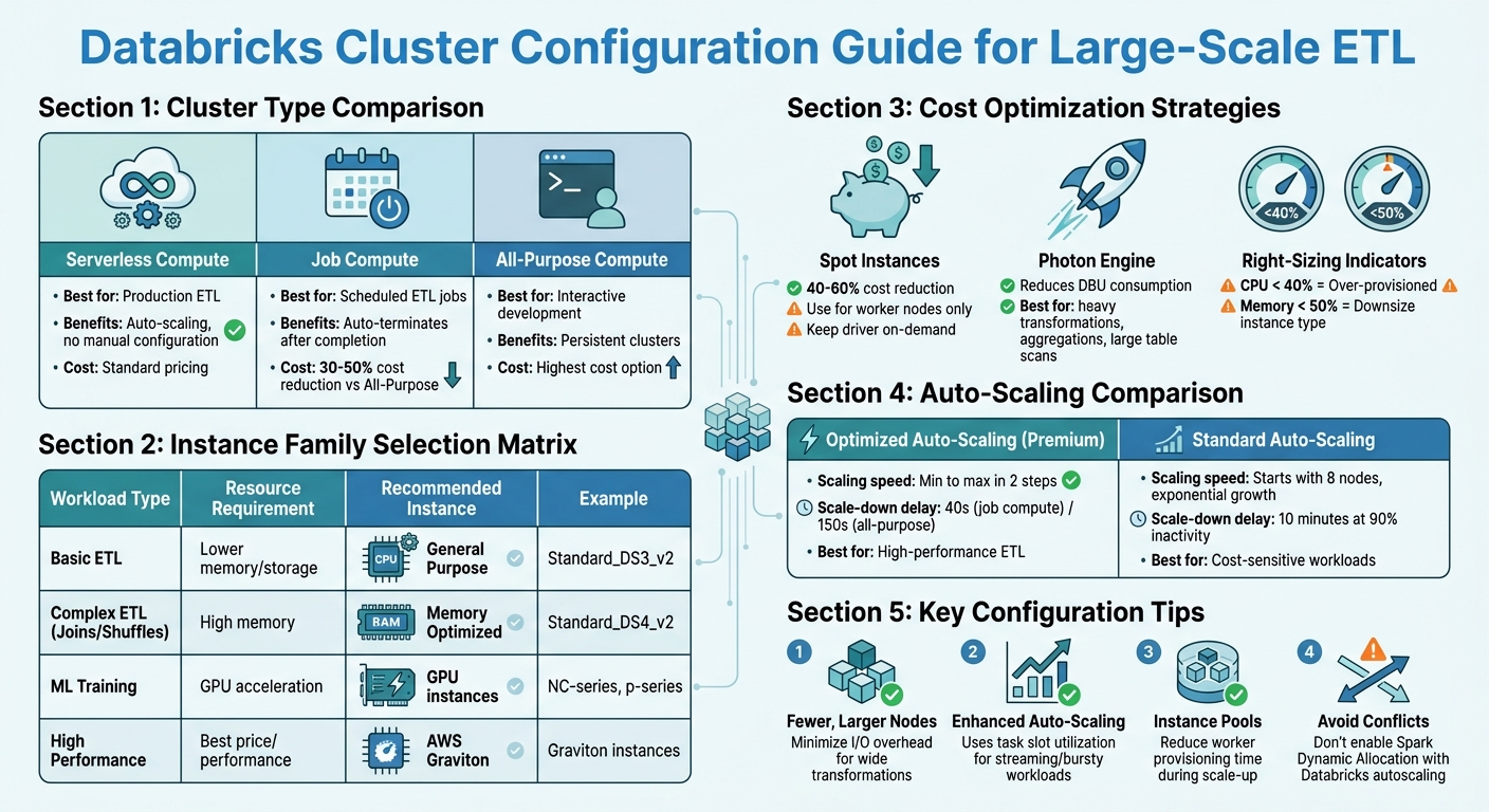
For production ETL, serverless compute is often the best option. It removes the need for manual configuration, scales automatically, and simplifies the process of sizing clusters. If serverless isn't suitable, Job Compute is a better alternative for scheduled ETL jobs compared to All-Purpose Compute. Job clusters are more cost-efficient, reducing expenses by 30-50%, and they automatically terminate once tasks are completed.

When choosing instances, focus on the total executor cores, memory, and local storage. For ETL tasks involving wide transformations like joins or unions, fewer but larger nodes can help minimize I/O overhead. If your CPU usage is consistently below 40%, your cluster is over-provisioned. Similarly, memory utilization below 50% suggests you could downsize your instance type.

Enable Photon for workloads that involve heavy transformations, aggregations, or large table scans. It improves resource allocation and reduces Databricks Unit (DBU) consumption. For batch ETL jobs, consider using spot instances for worker nodes to cut costs by 40-60%. However, keep the driver node on-demand to avoid cluster failures if spot capacity is reclaimed.

Workload Type	Resource Requirement	Recommended Instance Family
Basic ETL	Lower memory/storage	General Purpose (e.g., Standard_DS3_v2)
Complex ETL (Joins/Shuffles)	High memory	Memory Optimized (e.g., Standard_DS4_v2)
ML Training	GPU acceleration	NC-series or p-series
High Performance	Best price/performance	AWS Graviton instances

After selecting your cluster type and sizing, fine-tune performance using Databricks' autoscaling features.

Setting Up Auto-Scaling Policies

Databricks offers optimized autoscaling (available on Premium plans) and standard autoscaling, each with distinct behaviors:

• Scaling speed: Optimized autoscaling adjusts from minimum to maximum capacity in two steps, while standard autoscaling begins by adding eight nodes and scales exponentially.
• Down-scaling: Optimized autoscaling reduces nodes after 40 seconds of underutilization (for job compute) or 150 seconds (for all-purpose). Standard autoscaling requires 10 minutes of 90% inactivity before scaling down.

Set the min_workers value based on your workload patterns. For high-performance ETL, use a higher minimum to maintain baseline capacity and avoid delays when scaling up. For cost-sensitive tasks, set a low minimum (1-2 workers) and cap max_workers to prevent unexpected cost spikes. Attaching autoscaling clusters to instance pools can also reduce the time needed to provision workers during scale-up events.

For streaming or bursty batch workloads, enhanced autoscaling is ideal. It uses granular metrics like task slot utilization and task queue size instead of just CPU and memory usage.

These autoscaling settings help match computing resources to actual demand, keeping cloud costs under control. Important: Avoid enabling Apache Spark Dynamic Allocation (spark.dynamicAllocation.enabled) alongside Databricks autoscaling, as the two can conflict and lead to inefficient scaling decisions.

Batch Size and Trigger Optimizations

By default, Auto Loader processes up to 1,000 files per micro-batch. To manage resource usage effectively, use cloudFiles.maxBytesPerTrigger to set a soft limit on bytes processed per micro-batch and cloudFiles.maxFilesPerTrigger as a hard limit. Auto Loader will stop processing once either threshold is reached, preventing resource overloads.

For scheduled ETL tasks without low-latency needs, use Trigger.AvailableNow to process all files present at the start of the query. This reduces API calls and overhead. Avoid ProcessingTime or Continuous triggers in directory listing mode; instead, switch to file notification mode to cut down on API and discovery costs.

Enable Optimized Writes and Auto Compaction to address the issue of small files. For tables larger than 1 TB, schedule regular OPTIMIZE commands to consolidate data further. Databricks automatically adjusts target file sizes: for tables between 2.56 TB and 10 TB, the target file size increases linearly from 256 MB to 1 GB, and for tables over 10 TB, the target size is set to 1 GB. Additionally, configure cloudFiles.cleanSource with the MOVE or DELETE option to either archive or remove processed files. This speeds up file discovery and reduces storage costs.

Optimizing Data Storage with Delta Lake

Delta Lake offers powerful tools to streamline data storage and retrieval, working seamlessly with Databricks' large-scale ETL optimizations to improve pipeline efficiency.

Benefits of Delta Lake for Petabyte-Scale ETL

Delta Lake introduces ACID transactions to your data lake, ensuring consistency even when multiple jobs write to the same table simultaneously. This is especially important for large ETL pipelines where concurrent writes are common. Additionally, schema enforcement helps block corrupted or incompatible data from entering your tables, reducing errors further down the line and improving overall data quality.

Another key feature is built-in versioning, which allows you to "time travel" to previous data versions. This is incredibly useful for debugging failed ETL runs or recovering data overwritten by mistake. For operations at the petabyte scale, Delta Lake automatically gathers statistics - such as minimum and maximum values, null counts, and total record counts - for the first 32 columns of your table schema by default. These statistics enable data skipping, letting the query engine ignore irrelevant files and speeding up data retrieval.

Beyond these core features, advanced techniques like liquid clustering can take your data layout to the next level.

Liquid Clustering and Z-Ordering

Starting with Databricks Runtime 13.3, liquid clustering is the preferred method for organizing data on disk. As Avril Aysha explains, "Liquid clustering is the fastest and most efficient way to store your Delta Lake data on disk. It is more flexible and requires less compute than Z-Ordering and Hive-style partitioning".

Liquid clustering uses a tree-based algorithm to balance data layout automatically, cutting query times by over 40% in benchmarks. It works especially well with high-cardinality columns like customer_id or user_id. You can define up to four clustering keys and even change them later without requiring data rewrites.

For users on older runtimes or those with existing Z-Ordered tables, Z-Ordering still provides excellent results. This technique groups related data within the same files, reducing the amount of data scanned during queries. For instance, in one test with a billion-row dataset, Z-Ordering reduced query execution time from 4.33 seconds to just 0.6 seconds. In another example, applying Z-Ordering to a flight dataset with over 7 million records cut query time by about 70%, from 2 minutes to 39 seconds.

When implementing Z-Ordering, focus on columns most frequently used in WHERE clauses or join keys, and limit yourself to four columns to avoid reducing clustering efficiency. To maintain optimal performance, run OPTIMIZE ... ZORDER BY regularly, such as daily or weekly. Keep in mind that Z-Ordering and liquid clustering cannot be used simultaneously on the same table.

Pair these clustering methods with effective file management to further enhance query performance.

Data Skipping and File Management

Delta Lake's data skipping relies on metadata that describes each file's content. To maximize its benefits, include your most queried columns within the first 32 columns of your schema or adjust delta.dataSkippingNumIndexedCols to index additional columns.

For Delta Lake managed tables, Unity Catalog automatically adjusts file sizes to match the scale of your table, reducing the need for manual tuning. For tables larger than 1 TB, schedule regular OPTIMIZE commands to consolidate files if predictive optimization isn't enabled.

To save on compute costs, apply OPTIMIZE selectively by targeting the most recent partitions, such as the last seven days. After optimization, run VACUUM with a seven-day retention period to remove outdated files and reclaim storage space.

If you're using Unity Catalog managed tables, enable predictive optimization. This feature uses serverless compute to automatically perform OPTIMIZE and ANALYZE operations asynchronously, keeping your data layout optimized with minimal effort.

Performance Monitoring and Tuning in Databricks

Benchmarking ETL Performance

When it comes to monitoring ETL performance in Databricks, you need to focus on metrics at multiple levels: Application, Job, Stage, and Task. Among these, task-level metrics are the most revealing, helping you pinpoint bottlenecks like garbage collection delays, shuffle overhead, and disk spills.

The Spark UI is your go-to tool for diagnostics. It allows you to identify "straggler" tasks that slow down stages, visualize DAGs to locate costly shuffle operations (referred to as Exchanges), and track the progress of streaming queries. For persistent profiling data, Spark event logs are invaluable - they retain task-level insights even after a cluster is terminated.

"Spark event logs are the only universal source of task-level profiling data. Platform monitoring gives you node utilization and cost, but cannot tell you why a stage was slow." - Cazpian Docs

Databricks System Tables offer additional operational insights. For example:

• Use system.lakeflow to monitor pipeline health.
• Check system.billing to keep tabs on compute costs.
• Examine system.compute.node_timeline to analyze hardware usage patterns.

Keep an eye on these critical performance metrics:

Metric	Healthy Range	Action Required
GC Ratio	< 5%	> 10% (Increase memory or reduce cores)
Peak Memory	40% - 85%	< 40% (Over-provisioned); > 90% (OOM Risk)
Skew Ratio	< 2x	> 5x (Use salting or enable AQE)
Disk Spill	0 Bytes	> 0 Bytes (Increase executor memory)

For instance, a GC ratio under 5% is ideal, while anything over 10% indicates frequent pauses for garbage collection. Similarly, peak memory usage should stay between 40% and 85% - too low suggests over-provisioning, while exceeding 90% risks running out of memory.

These metrics form the foundation for the tuning strategies outlined below.

Iterative Spark Job Tuning

Start by enabling Adaptive Query Execution (AQE). This feature, activated by setting spark.sql.adaptive.enabled, automatically handles skewed joins and optimizes partitioning. A real-world example: In December 2025, Sahil Jain improved a Databricks pipeline that processed 7–8 billion rows. By enabling AQE, fine-tuning off-heap memory, and adjusting spark.sql.files.maxPartitionBytes to 256MB, his team cut runtime from 2 hours to 1 hour - a 35% improvement - without altering SQL logic.

For shuffle partition tuning, calculate the optimal number of partitions using the formula: Total Shuffled Data / 128MB. Ideally, each Spark task should handle around 128MB to 200MB of data. If disk spills show up in the Spark UI, increase spark.sql.shuffle.partitions to reduce the data size per task.

Data skew is another common issue, visible as a significant gap between the shortest and longest task durations. A skew ratio under 2x is acceptable, but anything above 5x signals severe imbalance. If AQE doesn't resolve the issue, try salting - adding random suffixes to distribute skewed keys more evenly across partitions.

For executor sizing, use the formula: recommended_memory = peak_JVM_heap x 1.15. A good balance for parallelism is 4–5 cores per executor, which minimizes garbage collection pressure while maintaining efficient intra-executor parallelism.

Pipeline Validation and Troubleshooting

Continuous monitoring is essential to maintain efficiency, especially at petabyte scale. In the Spark UI, watch for stages with high shuffle read/write values - these indicate heavy data movement and may require partition tuning. If you notice "Spill (Memory)" or "Spill (Disk)" warnings, consider increasing executor memory.

For streaming pipelines, track backpressure metrics to ensure your system can handle incoming data without delays. Query system.lakeflow logs to calculate average throughput (rows per second) and backlog (bytes or files). A stage becomes I/O bound if its data read/write per core exceeds ~3 MB/sec.

To assist the Cost-Based Optimizer, regularly run ANALYZE TABLE to refresh statistics. This helps Spark choose more efficient join strategies. Additionally, move complex logic and data type casts upstream of joins - this simple adjustment can cut query runtime by up to 40%. Avoid using standard Python UDFs due to their high serialization overhead; instead, rely on built-in Spark functions or Vectorized Pandas UDFs.

"Photon amplifies both good and bad execution plans. It doesn't hide inefficiencies; it exposes them faster." - Sahil Jain, Medium

For better log management, store cluster logs in Unity Catalog Volumes instead of DBFS. Use init scripts to convert Log4j logs to JSON format, making them easier to parse and analyze in AI or BI dashboards.

Implementing Predictive Optimization and Auto Loader

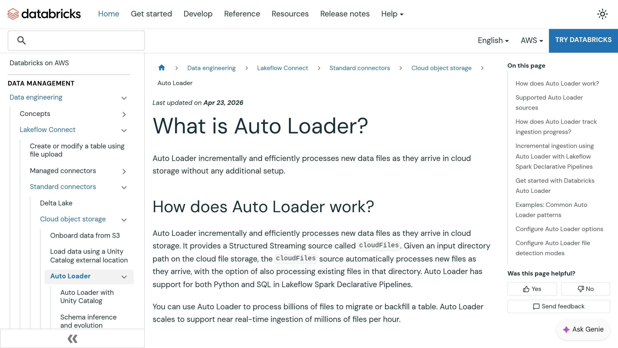
Using Auto Loader for Efficient Data Ingestion

Auto Loader takes the complexity out of handling massive data loads by continuously detecting and processing new files as they appear. For large-scale operations, file notification mode is a game-changer. It uses services like AWS SQS/SNS, Azure Event Grid, or GCP Pub/Sub to track new files, cutting down on the costs associated with repeatedly scanning directories for updates.

To ensure reliable ingestion, Auto Loader relies on a RocksDB checkpoint, which guarantees exactly-once processing. Starting with Databricks Runtime 15.4+, stream startup times have improved significantly by skipping the need to fully download the checkpoint state. To keep the checkpoint from growing indefinitely, it’s recommended to configure cloudFiles.maxFileAge to 90 days.

Managing the flow of data is just as important as ingesting it. Auto Loader offers rate limiting options to control the volume of data processed in each micro-batch, ensuring steady performance and protecting downstream systems.

Schema management is another standout feature. The new addNewColumnsWithTypeWidening mode (introduced in Runtime 16.4+) allows for seamless schema evolution, including changes like converting an int to a long, without requiring data rewrites. Auto Loader infers the initial schema by sampling up to 50 GB or 1,000 files. To avoid losing mismatched data, enabling the _rescued_data column captures any unexpected fields.

For cleanup, use cloudFiles.cleanSource to archive or delete processed files. Scheduling periodic runs in file notification mode also helps prevent directory clutter.

With data ingestion running smoothly, the next step is to utilize Predictive Optimization to streamline storage management and cut costs.

Predictive Optimization Techniques

Once data ingestion is set, Predictive Optimization takes over to handle storage maintenance for Unity Catalog managed tables. Since April 2026, this feature has been automatically enabled for all accounts. It uses an AI-driven engine to analyze query patterns and data layouts, ensuring optimizations are performed only when they’re worth the cost - typically consuming less than 5% of total ingestion costs.

This system replaces manual tasks like running ANALYZE commands with a stats-on-write approach, which is 7–10× faster than full table scans. Additionally, automatic statistics updates have led to up to 22% faster query performance by keeping column metadata up-to-date. The optimized VACUUM process uses the Delta transaction log instead of scanning directories, delivering up to 6× faster results at 4× lower costs.

For example, Anker’s data engineering team implemented Predictive Optimization and saw a 50% reduction in annual storage costs along with a 2× improvement in query performance. Shu Li, Data Engineering Lead at Anker, shared:

"Databricks' Predictive Optimizations intelligently optimized our Unity Catalog storage, which saved us 50% in annual storage costs while speeding up our queries by >2x".

File size tuning is another key feature. For tables over 10 TB, the system automatically adjusts the target file size to 1 GB to keep file counts manageable. For smaller tables (under 2.56 TB), a 256 MB target is used. Instead of manually configuring Z-ordering, Liquid Clustering selects the best clustering keys based on workload telemetry, further simplifying optimization.

You can track the effectiveness of these optimizations through the Data Governance Hub, which displays metrics like bytes compacted, clustered, vacuumed, and analyzed. For detailed insights, the system.storage.predictive_optimization_operations_history table logs operations, costs, and reasons for skipping certain tables. To avoid conflicts with the new optimization engine, it’s best to remove legacy settings like autoOptimize.autoCompact.

Conclusion and Next Steps

Key Takeaways

Optimizing Databricks ETL pipelines for massive datasets is a continuous engineering effort. The biggest performance gains often come from fine-tuning cluster configurations. For example, using the Photon Engine can lead to up to 12× faster performance on SQL-heavy tasks, while AWS Graviton instances offer a better price-to-performance ratio. Delta Lake improvements - such as switching to Liquid Clustering in newer runtimes - and automated maintenance with Predictive Optimization further enhance efficiency.

Managing shuffle and skew issues using Adaptive Query Execution (AQE) and salting techniques is critical for avoiding bottlenecks. Additionally, moving calculations out of join predicates and relying on native Spark SQL functions instead of Python UDFs ensures smoother execution. For incremental data loads, Auto Loader simplifies schema evolution and file notifications, making it a powerful tool.

A real-world example from August 2025 illustrates the impact of these strategies: Hanish Savla reduced the runtime of a production ETL pipeline from 10 hours to just 1 hour - a 90% improvement - by enabling the Photon runtime, implementing Z‑Ordering, and using Auto Loader. Optimizing ETL pipelines can lead to dramatic improvements in both speed and cost efficiency, but these results require hands-on practice to master.

Hands-On Training Resources

Practical training is key to turning these insights into real-world results. DataExpert.io Academy provides specialized programs in data engineering, analytics engineering, and AI engineering. These boot camps and subscriptions focus on tools like Databricks, Snowflake, and AWS, giving you the chance to apply optimization strategies to large-scale datasets through capstone projects.

• The All-Access Subscription costs $125/month (or $1,500/year) and includes over 250 hours of content, hands-on platform access, and a community to help tackle real-world ETL challenges.
• For a more structured learning path, the 15-week Data and AI Engineering Challenge costs $7,497 and features guest speaker sessions, mentorship, and a comprehensive capstone project.

Whether you're transitioning from visual ETL tools or sharpening your Spark tuning skills, these programs offer the code-first, iterative training needed to achieve measurable improvements in ETL performance.

FAQs

When should I use serverless compute vs. job clusters for ETL?

When dealing with workloads that are ad hoc, bursty, or unpredictable, serverless compute is a great choice. It allows for instant scaling and helps you avoid the costs associated with idle resources. On the other hand, job clusters are better suited for long-running, predictable ETL jobs, offering more control over resources and predictable costs.

In short, serverless compute excels in flexibility, while job clusters are ideal for handling consistent, resource-heavy tasks.

How do I choose the right shuffle partitions for petabyte-scale jobs?

When working with petabyte-scale jobs in Databricks, getting the right balance between parallelism and resource usage is key to optimizing shuffle partitions. Here's why: too few partitions can lead to memory issues, while too many partitions can pile on scheduling overhead, slowing everything down.

A good starting point is to set a high number of partitions - think several hundred - and then dive into the Spark UI to identify potential bottlenecks. Look out for signs like task skew or tasks taking unusually long to complete. These can indicate areas where adjustments are needed.

To make things even smoother, tap into adaptive query execution and skew handling. These features allow Databricks to adjust partitions dynamically during runtime, helping to fine-tune performance without manual intervention.

Should I use liquid clustering or Z-ordering on my Delta tables?

Liquid clustering tends to work better for optimizing Delta tables, especially when dealing with large and dynamic datasets. It automatically organizes the data, adjusts to changes, and handles high-cardinality filters or skewed data effectively. While Z-ordering can be helpful in certain scenarios, it demands more manual effort and lacks flexibility. For most petabyte-scale ETL pipelines, the self-tuning capabilities and performance advantages of liquid clustering make it the go-to option.