
ETL Pipeline Benchmarking: Metrics to Track
ETL pipelines are the backbone of modern data management, but their performance can degrade as data volumes grow and user demands increase. To keep pipelines running efficiently and cost-effectively, it’s essential to track the right metrics. Here’s what you need to focus on:
- Throughput and Data Volume: Measure how much data is processed (e.g., records per second) and track trends over time to identify bottlenecks.
- Latency and Freshness: Monitor how quickly data is processed and how current it is to meet Service Level Agreements (SLAs).
- Reliability and Data Quality: Track error rates, pipeline availability, and silent failures to ensure trustworthy data delivery.
- Resource Utilization and Costs: Analyze CPU, memory, and storage usage, as well as cost per run, to control cloud expenses.
- Scalability and Concurrency: Evaluate how well your pipeline handles increasing workloads and simultaneous processes without delays.
Mastering ETL Pipeline Optimization Techniques
sbb-itb-61a6e59
1. Throughput and Data Volume Metrics
Throughput is a key performance indicator for ETL pipelines. It measures the amount of data processed within a specific time frame, typically expressed as records per second or gigabytes per hour. To identify bottlenecks, track throughput separately for each stage - extraction, transformation, and loading. This approach ensures you can quickly pinpoint where performance issues arise.
"Slow ETL pipelines don't just delay dashboards – they stall every downstream decision that depends on fresh data." - Revanth Periyasamy, Data Engineer, Peliqan
Pay attention to backpressure by comparing the rate of incoming data to the processing rate. If the input rate exceeds the processing rate by a ratio greater than 1.2, your system is at risk of falling behind, potentially overwhelming downstream processes. Addressing this early can prevent widespread failures in your reporting workflows. For instance, switching from full-table refreshes to incremental loading can reduce processing time by 60–90%. Similarly, replacing row-by-row Python loops or SQL cursors with set-based SQL operations or vectorized libraries like Polars or DuckDB can accelerate transformation steps by 10–100x. During the loading phase, using bulk commands such as Snowflake’s COPY or PostgreSQL’s BULK INSERT can process batches of over 100,000 rows 5–10x faster than standard INSERT statements.
In addition to throughput, tracking data volume metrics is equally important. Monitor data volume alongside throughput to gain a more comprehensive view of pipeline health. Logging metrics like "rows in" vs. "rows out" at every stage helps detect silent data loss during filtering or transformation. Optimizing your extraction process by pruning unnecessary columns (instead of using SELECT *) can cut extraction time by 40–60%. To better understand long-term performance, store throughput trends in a time-series tool like Prometheus or CloudWatch. Single-run snapshots offer limited insight, but patterns over time can reveal crucial trends.
These throughput and data volume metrics are essential for keeping your ETL pipeline responsive and scalable.
2. Latency, Freshness, and SLA Metrics
Latency tracks how long operations take, while freshness measures how up-to-date the data is. These two metrics go hand-in-hand with throughput and data volume, offering a more complete picture of how well a pipeline performs. Latency looks at the duration of operations or the entire pipeline, while freshness focuses on the time gap between when a source event occurs and when it becomes accessible in the target system. A pipeline might have low latency but still deliver outdated data if the source feed is delayed or if no new data is processed.
This distinction plays a key role in setting Service Level Agreements (SLAs). Instead of relying on vague technical metrics like "DAG success rate", SLAs should be defined in terms of business needs. For instance: "Revenue data must be available within one hour of the source event." As one framework aptly states:
"An implicit SLA ('the revenue data is usually ready by 7 AM') is not an SLA - it is an expectation waiting to be violated." - Dataworkers
Clear SLA definitions enable precise measurement and accountability.
For batch pipelines, freshness should be calculated as the age of the most recent record in the target table. Use a formula like DATEDIFF(current_timestamp, MAX(loaded_at)). Avoid using the table’s modification timestamp since it updates even when no new data is added. If a business requires data by 8:00 AM, set the SLA for 7:00 AM to allow time for issue detection and resolution. For streaming pipelines, focus on metrics like consumer lag and the end-to-end latency from data ingestion to when it becomes available in the target system.
When analyzing latency, avoid relying on averages. Instead, monitor p95 and p99 percentiles to capture the slowest 1–5% of operations, which can quietly undermine user confidence. Little’s Law (Work in Progress = Throughput × Average Latency) illustrates why latency issues tend to spike as systems approach their capacity limits.
Data underscores the importance of these precise measurements. According to a 2024 Monte Carlo survey, only 28% of data teams have formal SLAs for freshness, completeness, or accuracy. Teams that adopt automated monitoring detect failures about 3.9 times faster - cutting the median time to detect from 47 minutes to just 12 minutes - and reduce SLA breaches for freshness from 4.2% to 1.1%. By focusing on latency and freshness, you can improve pipeline reliability and set clear expectations for timely data delivery. Advanced practitioners often pursue data engineering certifications to master these complex performance trade-offs.
Here’s a quick summary of benchmarks to aim for:
| KPI | 2026 Target | Red Flag Threshold |
|---|---|---|
| Data Freshness SLA Adherence | > 99% | < 95% |
| Mean Time to Detect (MTTD) | < 15 minutes | > 60 minutes |
| Mean Time to Resolve (MTTR) | < 120 minutes | > 480 minutes |
| On-Time Refresh Rate (Daily) | 95–99% | < 90% |
3. Reliability, Error, and Data Quality Metrics
Throughput and latency metrics might tell you how efficiently your pipeline operates, but error and quality metrics are what determine whether your data can actually be trusted. A pipeline can complete without any visible issues yet still deliver incomplete, duplicated, or corrupted data. These "silent failures" are particularly risky because they often go unnoticed for days, leaving stakeholders to make decisions based on flawed data.
"The first sign of a data integration problem is usually a data consumer asking 'why is this wrong' rather than any automated alert. Getting ahead of that requires monitoring at the record level, not just the process level." - Dennis Traina, Founder, 137Foundry
Focusing on record-level monitoring is essential for ensuring data quality. While process-level monitoring measures operational performance, it doesn’t catch the subtle errors that can undermine trust in your data. This distinction is critical because, in 74% of cases, business stakeholders are the first to spot data issues - not the data engineering team. And once a problem is identified, it’s not resolved quickly: as of 2026, the average time to fix a data incident has stretched to 15 hours, with 68% of teams spending over 4 hours just to detect the issue. The financial toll of poor data quality is staggering, costing companies an average of $12.9 million annually in penalties, rework, and lost opportunities.
To ensure reliability, it’s vital to implement robust quality controls. Start with multi-layered monitoring. For example, verify that record counts align across all stages - extract, transform, and load (ETL). If records fail at any stage, don’t discard them without notifying someone. Instead, route these records to a Dead Letter Queue (DLQ), which should log the original payload, the error message, and the stage where the failure occurred. A consistently growing DLQ signals a deeper issue, while occasional entries may just indicate isolated edge cases.
Beyond basic record counts, monitor for more nuanced issues like schema drift (unexpected changes to column names or data types), rising null values, and breaches of uniqueness constraints (e.g., duplicate primary keys). Instead of just counting errors, track error rates. A rate above 5% often indicates a systemic failure, while rates below 0.1% are generally linked to rare edge cases. Top-performing pipelines aim to keep error rates under 0.1%.
When error rates exceed acceptable thresholds or quality checks fail, it’s critical to act immediately. Trigger circuit breakers to halt downstream updates, preventing the spread of bad data. Leveraging machine learning for anomaly detection can also make a big difference, cutting detection times by 49% and reducing false positives by 37–42%.
Here are some key metrics to maintain data reliability:
| Reliability Metric | Target | Red Flag |
|---|---|---|
| Error Rate | < 0.1% | > 5% |
| Pipeline Availability | 99.9% | < 99% |
| Recovery Time | < 30 minutes | > 120 minutes |
| DLQ Growth Rate | Near zero | Consistently increasing |
| Stakeholder-Reported Issues | Rare | Recurring |
4. Resource Utilization and Cost Metrics
Reliability is just one piece of the puzzle; managing costs is equally important. Resource metrics help you connect operational performance to actual dollars, allowing you to identify inefficiencies before they escalate into budget issues.
To keep things organized, resource and cost metrics can be divided into three main categories: compute (vCPU hours, CPU utilization, throttling), memory (peak usage, spill to disk), and storage/network (data throughput and egress fees). For CPU utilization, aim for 70–80% sustained usage - anything lower suggests over-provisioning, while spikes to 100% could lead to job failures. Memory spill, on the other hand, is a major cost factor. When data exceeds available RAM, it spills over to slower local disk storage, which increases both runtime and compute expenses.
When it comes to cost metrics, it’s better to focus on specifics rather than just tracking total monthly spend. Metrics like cost per successful run and cost per GB processed are much more actionable. These unit-based metrics quickly highlight inefficiencies as data volumes grow. As BigData Boutique explains:
"The loudest job is rarely the most expensive one. Without cost-per-run telemetry, teams tune the pipeline that pages them, not the one that is quietly costing six figures a year."
Two common culprits for inflated costs are data skew and small files. Data skew happens when one partition holds a disproportionate amount of rows, causing a single cluster node to remain active long after others have finished - resulting in unnecessary charges. Similarly, the small-file issue arises when engines spend more time opening numerous small files rather than processing data, driving up compute costs without improving throughput. Solutions like compaction and predicate pushdown (filtering rows and columns at the source) are effective at addressing these inefficiencies. Aspiring engineers can learn these optimization techniques in a data engineering boot camp designed for career readiness.
Infrastructure inefficiencies are another area to watch. These can account for up to 32% of wasted cloud spending, often due to clusters that don’t auto-terminate or warehouses sized for peak loads that never materialize. Implementing auto-suspension for idle clusters and running stateless batch workloads on spot or preemptible instances can reduce compute costs by 60–90%. Tools like Databricks System Tables, AWS CloudWatch, and the Spark History Server provide the detailed insights needed to monitor these metrics and take action.
Here’s a quick reference table for key metrics:
| Metric | What It Measures | Target |
|---|---|---|
| CPU Utilization | Active compute vs. provisioned capacity | 70–80% sustained |
| Memory Spill to Disk | Data overflow from RAM to local storage | Minimize; high spill = undersized cluster |
| Cost per Successful Run | Total spend (compute + storage + egress) per completed job | Trending flat or down as volume grows |
| Network Egress Fees | Cross-region or cross-AZ data transfer costs | Track separately; can add 15–30% to raw ingest spend |
| Cluster Idle Time | Uptime with no active processing | Near zero; implement auto-termination for idle clusters |
5. Scalability, Elasticity, and Concurrency Metrics
Once you've optimized costs, the next challenge is ensuring your pipeline can handle increasing data and workloads without breaking a sweat. After all, cost efficiency doesn't mean much if your system collapses under pressure.
One of the clearest indicators of scalability is the linear scaling factor - how much performance improves when you add more workers. Ideally, doubling the number of workers should cut runtime in half. But in reality, coordination overhead often limits this to around 60–80% efficiency. As Revanth Periyasamy explains:
"Parallel ETL achieves near-linear scalability up to the point where I/O, network, or shared resources become the bottleneck. In practice, teams report 60–80% linear scaling."
Scalability isn't just about adding workers; it also means monitoring how well your system handles concurrent workloads. Keep an eye on the backpressure ratio, which measures the balance between input and processing rates. If this ratio climbs above 1.2, delays can pile up. Similarly, watch consumer lag in systems like Kafka. If lag grows during high-volume periods instead of stabilizing, your pipeline isn't elastic enough to handle bursts.
Another hidden threat to scalability is data skew - when one partition ends up with significantly more rows than others. This imbalance can cause a single node to lag and delay the entire process. As Devtools.cloud notes:
"Most optimization failures happen when one 'fast' stage hides a single pathological straggler that drags the whole DAG past the SLA."
To avoid this, flag any task that takes more than 10× the median completion time.
While scalability ensures your pipeline performs under heavy loads, concurrency management prevents resource conflicts. For example, one team's large backfill job could hog resources, leaving critical tasks starved. Metrics like queue_wait_seconds can help identify these issues early. To safeguard key workloads, set concurrency caps or use tools like Airflow pools for prioritization. It's also a good idea to periodically stress-test your pipeline with 10× your current data volume to uncover potential bottlenecks before they become production issues.
| Metric | What It Measures | Target |
|---|---|---|
| Linear Scaling Factor | Performance gain per added worker | 60–80% efficiency |
| Backpressure Ratio | Input rate vs. processing rate | Keep below 1.2 |
| Consumer Lag | Delay between data arrival and processing | Stable or decreasing during volume spikes |
| Task Skew | Variance in individual task completion times | No task should take >10× the median |
| Queue Wait Seconds | Time a task waits for an available worker slot | Minimize; high values signal resource contention |
Comparison Table
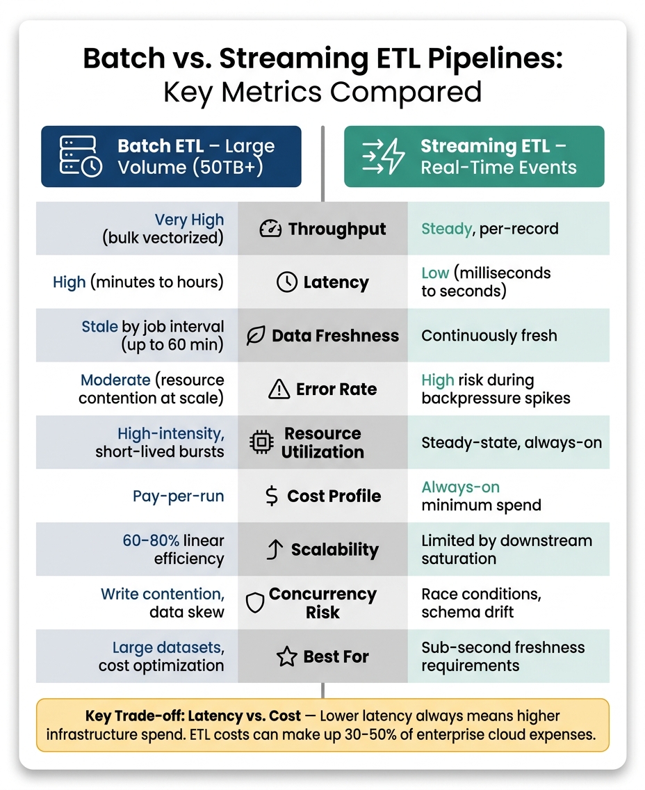
Batch vs. Streaming ETL Pipelines: Key Metrics Compared
The table below offers a clear side-by-side comparison of batch and streaming ETL pipelines, highlighting the trade-offs between them. This can help you weigh the strengths and weaknesses of each approach depending on your specific needs.
For example, a batch pipeline handling 50 TB of financial data overnight will have different priorities than a streaming pipeline designed for real-time fraud detection.
| Metric | Batch ETL (Large Volume, e.g., 50TB+) | Streaming ETL (Real-Time Events) | Key Trade-off |
|---|---|---|---|
| Throughput | Very high (bulk vectorized processing) | Steady, per-record | Batch focuses on processing large volumes; streaming prioritizes continuous processing |
| Latency | High (minutes to hours) | Low (milliseconds to seconds) | Lower latency demands higher infrastructure costs |
| Data Freshness | Stale by job interval (up to 60 min) | Continuously fresh | Achieving continuous freshness comes with 24/7 compute costs |
| Error Rate | Moderate (resource contention at scale) | High risk during backpressure spikes | Errors in streaming can escalate quickly under heavy load |
| Duplicate Rate | High risk without idempotency logic | High risk during retries/offset resets | Both need careful handling (MERGE/UPSERT); auditing is tougher in streaming |
| Resource Utilization | High-intensity, short-lived bursts | Steady-state, always-on | Batch scales down to zero; streaming maintains constant base usage |
| Cost Profile | Pay-per-run | Always-on minimum spend | ETL costs can make up 30–50% of enterprise cloud expenses |
| Scalability | Linear scaling up to 60–80% efficiency | Limited by downstream saturation | A backpressure ratio >1.2 indicates streaming is overwhelmed |
| Concurrency Risk | Write contention, data skew | Race conditions, schema drift | Both require task isolation and idempotent writes to avoid conflicts |
This breakdown underscores the primary trade-off: latency versus cost. As Kestra explains:
"The biggest mistake in choosing between the two is assuming lower latency is always better. It is not, because latency has a cost."
For large datasets (50–100 TB), batch processing is the go-to for optimizing throughput and keeping costs manageable. On the other hand, serverless options are better suited for real-time, lower-volume workloads.
If you can tolerate a slight delay, batch processing is simpler and more cost-effective. Use streaming pipelines only when sub-second data freshness is absolutely necessary. Alternatively, micro-batching (every 10 seconds to 5 minutes) offers a middle ground, balancing data freshness with operational simplicity.
Conclusion
Regular benchmarking is key to keeping your data infrastructure running smoothly and staying one step ahead of potential challenges. It’s not just about monitoring - it’s about turning those observations into actionable changes.
For instance, organizations that prioritize ETL pipeline optimization have seen impressive results: cutting average data latency by 55% and trimming cloud expenses on data movement by up to 35%.
"You cannot improve what you do not measure." - Revanth Periyasamy, Peliqan
It’s also important to balance the metrics you track. Pair core metrics like cost per run and throughput with guardrail metrics such as SLA breach rate or data freshness. This ensures that gains in one area don’t come at the expense of another. Without this balance, teams risk focusing on the wrong priorities.
If you're ready to put these ideas into action, check out the programs from DataExpert.io Academy. Their boot camps and self-paced courses cover hands-on training with tools like Apache Spark, Databricks, Snowflake, and AWS, helping you bridge the gap between understanding metrics and applying them effectively in production.
FAQs
Which ETL metrics should I track first?
To get started, keep an eye on key metrics to set a baseline. Begin by comparing record counts at every stage of the process - records going in should match the sum of records coming out, skipped, or flagged as errors. Pay particular attention to three main areas:
- Throughput: How many records are processed within a given time frame.
- Latency: The time it takes to complete each stage.
- Error Rates: Both the total number of errors and the rate per thousand records.
Tracking these metrics can uncover bottlenecks and ensure your pipeline stays in good shape.
How do I measure data freshness correctly for batch vs. streaming pipelines?
Measuring how up-to-date your data is depends on the type of pipeline you're working with.
For batch pipelines, you can evaluate freshness by checking the time difference between when a job was scheduled to run and when it actually finished. Another approach is to measure the time that has passed since the last data load.
For streaming pipelines, focus on metrics like end-to-end latency - essentially, how long it takes for an event to move from its creation point to being available at the sink. You should also keep an eye on consumer lag, which tracks how far behind consumers are in processing the latest data.
To get precise insights, you can run SQL queries to calculate metrics such as delay or P95 latency, which provide a clear view of your pipeline's performance.
What’s the fastest way to catch silent data loss in my ETL pipeline?
Detecting silent data loss effectively requires more than just monitoring job statuses. Even when jobs appear successful, data can still be corrupted or incomplete. This is where automated data observability comes into play - it helps uncover issues that traditional monitoring might miss.
Here are some key strategies to enhance data observability:
- Track row count anomalies: Compare current row counts to historical baselines to spot unexpected changes.
- Validate statistical distributions: Check metrics like mean and variance to ensure data integrity.
- Leverage dead letter queues (DLQs): Use DLQs to capture and flag records that fail processing.
- Deploy anomaly detection: Monitor metrics such as data freshness and completeness to identify irregularities.
By adopting these practices, you can stay ahead of potential data issues and ensure your pipelines deliver accurate and reliable results.