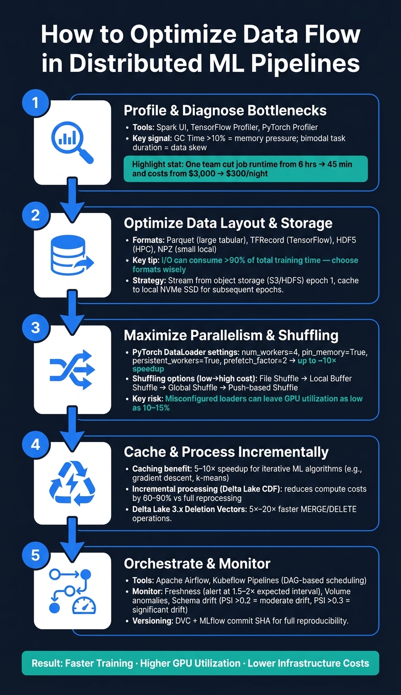
How to Optimize Data Flow in Distributed ML Pipelines

Optimizing data flow in distributed ML pipelines is crucial to ensuring efficient training and reducing costs. The biggest challenge? Data preparation often becomes a bottleneck, leaving GPUs underutilized and slowing down workflows. This guide dives into actionable strategies to resolve these issues and improve pipeline performance and master data engineering concepts.

Key Takeaways:

1. Profiling Bottlenecks: Use tools like Spark UI, TensorFlow Profiler, or PyTorch Profiler to identify slow stages and inefficiencies.
2. Data Layout & Storage: Optimize formats (e.g., Parquet, TFRecord) and balance between object storage and local SSDs for faster I/O.
3. Parallel Loading & Shuffling: Configure data loaders and shuffling methods to maximize GPU utilization and ensure even data distribution.
4. Caching & Incremental Processing: Reduce redundant computations with caching and process only new or updated data for efficiency.
5. Orchestration & Monitoring: Use tools like Airflow or Kubeflow to schedule tasks and monitor data freshness, volume, and schema integrity.

By addressing these areas, you can achieve faster training times, higher GPU utilization, and lower costs.

Overcoming Distributed ML Challenges with Ray Train | Ray Summit 2024

sbb-itb-61a6e59

Profiling and Diagnosing Data Bottlenecks

Before diving into code modifications, it’s critical to profile your pipeline to identify where time is being wasted. Skipping this step is a common pitfall in distributed machine learning workflows. Without profiling, you risk optimizing the wrong part of the pipeline and seeing no improvement. The objective is simple: pinpoint the slowest stage with evidence, not guesswork.

Using Profiling Tools

Several tools can help you analyze and diagnose bottlenecks effectively:

• Spark UI: Perfect for data-heavy transformations and shuffle operations. Use the Stages tab to detect data skew and shuffle costs, the SQL tab to examine execution plans, and the Executors tab to monitor memory usage. A key indicator here is GC time - if it exceeds 10% of total task duration, your executor heap may be under pressure due to over-caching or excessive object creation.
• TensorFlow Profiler: Tailored for deep learning workflows, this tool’s Input Pipeline Analyzer reveals whether your model is input-bound (i.e., the GPU is idle, waiting for data). The Trace Viewer provides a detailed view of operation durations across host and device, helping you locate delays between training steps.
• PyTorch Profiler: Particularly useful in distributed training setups like Ray Train. It identifies communication bottlenecks, memory leaks, and inefficiencies in kernel execution - essential for debugging multi-GPU environments.

Here’s a quick reference table of metrics, tools, and common issues:

Metric	Tool	Warning Threshold	Likely Issue
GC Time	Spark UI	> 10% of task duration	Memory pressure
Shuffle Spill (Disk)	Spark UI	Any non-zero value	Insufficient executor memory
Fetch Wait Time	Spark UI	High relative to compute	Network bottleneck
Input Bound %	TF Profiler	High device idle time	Slow data ingestion
Scheduler Delay	Spark UI	Consistently high	Too many small tasks

Step-by-Step Bottleneck Diagnosis

Begin by ranking your pipeline stages by duration and isolating the longest-running one. Then, examine the task count for that stage. If there’s only a single task, it could indicate limited parallelism or a non-partitionable data source. On the other hand, a bimodal task duration histogram - where most tasks complete quickly but a few take significantly longer - often points to data skew. This is frequently caused by a "hot key" that represents a disproportionate share (10% or more) of the total records.

For example, in April 2026, Isabel, a senior data engineer at a financial institution, used this method to troubleshoot a transaction risk feature pipeline that was costing $81,000 more per month than expected. By analyzing the Spark UI, she uncovered severe data skew during a merchant category join, excessive shuffle volumes, and garbage collection consuming nearly half of executor time. After addressing these issues, the job runtime dropped from 6 hours to just 45 minutes, slashing nightly costs from $3,000 to $300.

When working with GPU training pipelines, try replacing your real dataset with synthetic data. If training speeds up significantly, the bottleneck lies in your data input pipeline - not the model or hardware.

"A machine learning pipeline is not a function. It is a chain of distributed transformations, each with its own dependencies, its own timing characteristics, and its own failure modes." - Samuel Desseaux, Erythix

Optimizing Data Layout and Storage

Once you've identified your bottlenecks, the next step is to refine your data storage and structure. Poorly designed data formats or storage systems can make input/output (I/O) the biggest expense in your workflow - sometimes consuming over 90% of total training time. This phase builds on your earlier analysis, focusing on reorganizing data to improve efficiency and throughput.

Choosing the Right Data Formats and Storage Options

The efficiency of a data format in distributed machine learning depends on your framework, dataset size, and how you access the data. Here's a breakdown of some commonly used formats:

Format	Best For	Key Advantage	Watch Out For
Apache Parquet	Large-scale tabular data (tens of TBs)	Columnar storage, supports projection/filter pushdown	CPU-heavy PyArrow-to-NumPy conversions
TFRecord	TensorFlow training pipelines	High bandwidth for sequential reads	Limited to TensorFlow workflows
HDF5	HPC and scientific workloads	Balanced performance, shared multi-process access	Complex metadata handling
NPZ	Small, local projects	Seamless NumPy integration	No optimizations for distributed I/O

For large-scale distributed training, Parquet is often the go-to format. However, converting PyArrow data to NumPy tensors can strain your CPU, especially if done on the main training thread. A better approach is to offload these transformations to worker threads. This ensures the conversion process runs in parallel, keeping your GPU busy and reducing overall training time. Such adjustments not only speed up workflows but also cut compute costs.

When it comes to storage infrastructure, there’s a trade-off between object storage (e.g., S3, HDFS) and local SSDs. Object storage offers scalability and cost efficiency but is network-dependent, while local SSDs are faster but have limited capacity. A practical compromise is to stream data from object storage during the first epoch and cache preprocessed data on local NVMe SSDs (e.g., /tmp) for subsequent epochs. This eliminates redundant network I/O in later stages.

Improving Data Transfer Efficiency

After optimizing data formats, the next step is to streamline data transfer methods. Reducing data movement and transfer distances often yields better results than upgrading hardware.

Co-locating storage with compute is a straightforward way to cut I/O delays. By running tasks on the same node where the data resides, you can avoid inter-node transfers entirely. For example, in Ray Data, you can configure execution settings to prioritize placing read tasks on the same node as the consumer.

Compression is another key factor. Fast-decompression formats like Snappy strike a balance between size reduction and speed, making them ideal for training pipelines. On the other hand, Gzip provides better compression ratios but demands more CPU resources, making it more suitable for archival purposes than active training reads.

Dataset sharding is equally important. Dividing your dataset into smaller shards allows for parallel reads, significantly increasing throughput. When using Parquet, combine sharding with projection pushdown (reading only the necessary columns) and filter pushdown (skipping irrelevant rows during scans) to minimize the amount of data loaded into memory. For streaming workloads, aim to keep individual data blocks between 1 MiB and 128 MiB. Smaller blocks can lead to excessive scheduler overhead, while larger ones may increase latency.

"Spending extra on FSx for Lustre often saves money - it shortens the total training time, reducing the total bill despite the higher storage cost." - Blessy Moses, DevEx Advocate

This insight underscores a critical point: optimizing your storage setup isn't just about performance - it directly influences your infrastructure expenses. Efficient data handling can lead to faster training cycles and lower overall costs.

Increasing Throughput with Parallelism and Data Shuffling

After optimizing storage, the next challenge is ensuring data is loaded and distributed fast enough to keep GPUs fully utilized. Two key strategies - parallel data loading and effective shuffling - can significantly bridge the gap between your hardware's potential speed and its actual performance.

Configuring Parallel Data Loading

Misconfigured data loaders can drastically limit GPU utilization, sometimes as low as 10–15%. To address this, frameworks like PyTorch, TensorFlow, and Ray Data offer tools to streamline data loading.

In PyTorch, the DataLoader provides several options to improve throughput:

• num_workers: Start with 2–4 workers per GPU and adjust gradually. Too many workers can cause CPU contention.
• pin_memory=True: Enables faster CPU-to-GPU data transfers using Direct Memory Access (DMA).
• persistent_workers=True: Reduces overhead by keeping worker processes alive across epochs.
• prefetch_factor=2: Allows the CPU to prepare the next batch while the GPU processes the current one, overlapping computation with I/O.

When these settings were combined - such as num_workers=4, prefetch_factor=2, pin_memory=True, and persistent_workers=True - benchmarks showed up to a ~10× speedup compared to a single-process baseline.

For TensorFlow, use .prefetch(tf.data.AUTOTUNE) and num_parallel_calls=tf.data.AUTOTUNE to dynamically adjust thread counts. Similarly, in Ray Data, the parallelism parameter (e.g., ray.data.read_parquet(path, parallelism=1000)) controls the number of concurrent read tasks.

"The GPU wasn't slow – it was starving. DataLoader workers generated 200,000 CPU context switches... leaving the GPU waiting an average of 301ms per data transfer." - David Mail, Co-Author of Ingero

This quote underscores a critical but often overlooked issue: excessive CPU context switching can quietly degrade pipeline performance, even when GPU utilization appears low.

Once your data loader is optimized, the next step is ensuring balanced data distribution across workers.

Shuffling Data for Even Load Distribution

Parallel data loading alone isn’t enough - data must also be shuffled effectively to prevent uneven workloads and ensure balanced training. This is a core skill for those breaking into data engineering. The choice of shuffling method depends on your model's need for randomness and the scale of your dataset. Here’s a quick comparison:

Shuffling Method	Randomness Quality	Cost	Best Use Case
File Shuffle	Low	Very Low	Fast ingestion (metadata-only)
Local Buffer Shuffle	Medium	Moderate	Balancing randomness and throughput
Global Shuffle	High	High	Order-sensitive models (e.g., tabular data)
Push-based Shuffle	High	Scalable	Large datasets (over 1 TB or 1,000 blocks)

For most workloads, local buffer shuffling strikes a good balance. It randomizes rows in memory without introducing the high costs of cross-node data transfers. Save global shuffling for cases where your model is highly sensitive to data order, as it forces the entire dataset to be materialized, which can be expensive.

"The more global the shuffle is, the more expensive the shuffling operation. The increase compounds with distributed data-parallel training on a multi-node cluster due to data transfer costs." - Ray Data Performance Tips

If you’re working with Spark pipelines, the default spark.sql.shuffle.partitions value of 200 is often suboptimal. Adjust this to match your cluster's core count. For small lookup tables (under 100 MB), use broadcast() joins to bypass shuffle operations entirely. When data skew is an issue - where a few keys dominate the distribution - apply salting (adding a random prefix to skewed keys) to balance the load across partitions.

Finally, if you’re caching data, always shuffle after caching to ensure re-randomization for each epoch.

Caching and Incremental Processing

After parallel loading and shuffling, redundant computation often becomes the next major hurdle.

Applying Caching in ML Pipelines

Spark's lazy execution model can lead to repeated work. Every time you run an action like count(), show(), or write(), Spark re-executes the entire DAG from scratch. For iterative machine learning algorithms like gradient descent or k-means, this means reloading and reprocessing your training data for every iteration. By caching the training DataFrame, you reduce each iteration to a quick in-memory scan, which can speed up training by 5–10 times.

Caching is particularly effective in "Diamond DAG" scenarios, where a single preprocessed DataFrame splits into multiple downstream pipelines. Instead of recalculating the same transformations for each branch, you compute them once and reuse the results.

When you call .cache(), it’s important to remember that caching is lazy - it won’t take effect until you trigger an action like .count() to materialize the cache across the cluster. For large datasets on clusters with limited memory, use MEMORY_AND_DISK_SER combined with the Kryo serializer. This approach is 3–5 times more memory-efficient than deserialized storage and automatically falls back to disk if memory is exhausted. To avoid memory leaks or eviction issues in long-running jobs, always follow up with .unpersist() once the cache is no longer needed.

"Caching in Spark is lazy and partition-level - understanding how StorageLevel and eviction work is the difference between a speedup and an OOM." - Abstract Algorithms

On Databricks, the built-in disk cache complements manual Spark caching by storing repeated Parquet and Delta reads on fast SSDs at worker nodes. This feature is especially useful for query-heavy workloads.

Once redundant computations are addressed through caching, the next step is to focus on processing only new or updated data.

Implementing Incremental and Real-Time Processing

Building on the efficiencies of caching, incremental processing avoids re-running the entire pipeline by targeting only new or modified records. This approach can reduce compute costs by 60–90% compared to full reprocessing.

For Delta Lake pipelines, enabling the Change Data Feed (CDF) is one of the most effective strategies. CDF tracks row-level changes - like inserts, updates, and deletes - in a separate log, allowing your pipeline to process only the changes since the last run. This eliminates the need for costly full-table scans. Delta Lake 3.x further enhances performance with Deletion Vectors, which improve MERGE and DELETE operations by 5x to 20x by avoiding full file rewrites. For scheduled batch jobs, using trigger(availableNow) lets you leverage Spark Structured Streaming’s state management and exactly-once guarantees without the overhead of a continuously running cluster.

One common issue with incremental writes is the "small file problem", where frequent updates generate too many small files, slowing down queries due to excessive metadata processing. To address this, schedule daily OPTIMIZE jobs for recent partitions (e.g., WHERE date >= current_date - 7) and perform a weekly full-table OPTIMIZE with Z-ORDER on high-cardinality columns to maintain efficient performance.

"Optimization is not about writing clever code - it is about understanding how Spark and Delta Lake work physically." - Naveen Vuppula, Senior Data Engineering Consultant, DriveDataScience

Orchestrating and Monitoring Distributed ML Pipelines

Building on earlier discussions about caching and incremental processing, effective orchestration ensures your data pipelines run smoothly. This means tasks execute in the correct order, stay on schedule, and recover reliably when issues arise.

Workflow Orchestration with DAGs

Orchestration tools like Apache Airflow and Kubeflow Pipelines use Directed Acyclic Graphs (DAGs) to structure workflows. For instance, tasks like feature engineering won't start until data ingestion has successfully completed.

In machine learning workflows, using KubernetesExecutor allows you to spin up isolated pods with dedicated GPU access and custom dependencies. However, this approach comes with a cold start delay of 15–60 seconds per task due to pod scheduling and container startup.

"Training should not run on an Airflow worker... the correct approach is to run training in an isolated Kubernetes pod." - EngineersOfAI

Some best practices for Airflow include:

• Setting max_active_runs=1 to avoid GPU resource conflicts during concurrent retraining.
• Using mode="reschedule" for sensors to release worker slots between checks while waiting for upstream data.
• Avoiding large DataFrames in XCom; instead, store data externally and pass file paths through XCom.

Airflow also supports data-aware scheduling via Datasets. For example, you can trigger training DAGs automatically when an upstream ETL process writes to a specific S3 path. This scheduling structure ensures predictable training cycles and aligns well with earlier pipeline performance optimizations.

Once tasks are orchestrated, the next step is monitoring their execution and ensuring data integrity.

Monitoring and Alerting for Pipeline Health

While orchestration ensures tasks execute as planned, monitoring focuses on verifying that data arrives correctly and remains consistent. Key areas to monitor include:

• Freshness: Set alerts for 1.5 to 2 times the expected update interval to minimize false alarms.
• Volume: Keep an eye on data size to catch anomalies.
• Schema and Distribution: Track schema changes and metrics like the Population Stability Index (PSI). A PSI above 0.2 suggests moderate drift, while values above 0.3 indicate significant drift.
• Lineage: Ensure clear traceability of data sources.

Each alert should link to a runbook with specific triage steps and recovery commands. Routing alerts to the right team can also reduce alert fatigue and speed up issue resolution.

Data Lineage and Versioning

Robust data lineage and versioning are essential for reproducibility in ML pipelines. Knowing exactly which data was used for training ensures transparency and consistency. Tools like DVC manage lightweight Git-tracked metafiles alongside remote storage, while lakeFS provides Git-style branching directly on your object store - ideal for large-scale data lakes.

To maintain reproducibility:

• Pass a specific commit SHA during training to ensure consistent datasets.
• Log this commit hash in MLflow to create a traceability chain that links the production model to the exact training run and dataset version.

For regulated industries, extend traceability to individual records. For example, include a structured manifest within the versioned dataset to answer questions like, "Was patient PAT-00023 included in this model?" This level of detail is crucial for compliance with regulations like GDPR and HIPAA.

Conclusion and Next Steps

Improving every layer of your data pipeline is the key to creating scalable, distributed machine learning (ML) systems. Optimizing data flow in these pipelines involves a series of targeted enhancements, from profiling to orchestration. Each improvement builds on the previous one, creating a smoother and more efficient process.

The benefits of these optimizations are clear. Poorly designed pipelines can result in GPUs operating at just 10–15% capacity, wasting valuable hardware resources. By addressing inefficiencies systematically, you can transform a fragile pipeline into a reliable, high-performing system.

As Ujjwal Sharma from IIT Bombay puts it:

"The ultimate competitive advantage in modern AI is the ability to execute flawless, end-to-end systems engineering across all layers of the hardware and software pipeline."

Now it’s time to put these strategies into action. If you’re looking to deepen your skills, DataExpert.io Academy offers hands-on programs tailored to distributed systems. For instance:

• The Data Engineering Boot Camp ($3,000) is a 5-week course covering advanced topics like Spark shuffle joins, memory tuning, and partitioning.
• The All-Access Subscription ($125/month) provides over 250 hours of self-paced content, focusing on tools like Apache Spark, Databricks, Delta Lake, Apache Iceberg, and Airflow. Subscribers also gain immediate cloud access to platforms like Databricks, AWS, and Snowflake for practical learning.

If you’re not ready to commit financially, you can start with the free Data Engineer Handbook on GitHub. With over 41,500 stars, it’s packed with roadmaps, project ideas, and beginner boot camps to help you establish a strong foundation in data engineering.

FAQs

How do I know if my GPUs are input-bound?

To determine if your GPUs are being held back by input issues, look for signs of GPU starvation - this happens when the GPU sits idle, waiting for data to process. Key indicators include:

• Low or inconsistent GPU utilization: Utilization may appear bursty or irregular.
• Idle periods between kernel executions: Gaps in activity suggest the GPU is waiting for input.
• High CPU usage: The CPU might be working overtime to feed data to the GPU.

You can use tools like PyTorch Profiler or TensorBoard to pinpoint gaps in your training workflow. For a more thorough check, try testing with synthetic data or leverage NVIDIA Nsight Systems to confirm if input bottlenecks are causing delays.

When should I use global shuffle vs local buffer shuffle?

Global shuffle guarantees top-tier randomness, which is crucial for tasks like training models on tabular data. However, this approach demands significant resources, including high network bandwidth, disk usage, and memory. It’s best suited for scenarios where your model requires precise randomization, and your infrastructure can handle the added strain.

On the other hand, local buffer shuffle is a faster, more resource-friendly option. It shuffles data within smaller batches, making it ideal for massive datasets or when global shuffling isn’t feasible. If local processing provides enough randomness for your needs, this method can save time and costs.

What’s the safest way to cache data without running out of memory?

To safely cache data in distributed machine learning pipelines, it's important to use a bounded memory strategy. Keep memory utilization under 80% to reduce the risk of eviction pressure. For added reliability, consider using a layered storage approach, such as Spark's MEMORY_AND_DISK, which allows data to spill over to disk when memory capacity is exceeded.

Additionally, implement request coalescing to avoid redundant recomputation, which can save both time and resources. To handle stale data efficiently, use time-to-live (TTL) settings combined with staleness budgets, ensuring outdated data is managed without disrupting your workflow.