
Snowflake Query Tuning: Best Practices for Low Latency
When your Snowflake dashboards take 45 seconds to load, or your API response times are inconsistent, it's not just frustrating - it’s a problem that impacts performance and costs. While Snowflake offers a powerful architecture, achieving low latency requires understanding and optimizing key factors like query structure, warehouse configurations, and data layout.
Here’s the gist:
- Optimize compute: Right-size your warehouse to avoid memory spills and queuing.
- Improve storage: Use clustering keys and efficient data layouts to reduce partition scans.
- Write better SQL: Filter early, avoid unnecessary columns, and leverage caching.
How Snowflake Executes Queries

Snowflake Architecture and Query Lifecycle
Snowflake’s architecture is built on three distinct layers, each playing a critical role in query execution:
- Cloud Services Layer: This is where queries are parsed, user privileges are verified, and optimizations like pushdown filtering are applied to eliminate unnecessary rows early in the process.
- Virtual Warehouse Layer: Here, the actual execution takes place, including reading data, processing joins, and performing aggregations.
- Storage Layer: Data is stored in immutable, columnar micro-partitions (ranging from 50 to 500 MB each) that include metadata like minimum and maximum values, as well as distinct counts. This metadata is key to partition pruning, which allows Snowflake to skip irrelevant partitions and speed up query execution.
Once a query is executed, its results are cached in the Result Cache for 24 hours. If the same query is run again within that window, the cached result is returned instantly, saving warehouse credits. Additionally, the Local Disk Cache stores decompressed data on the warehouse’s SSD nodes, making repeated access faster than fetching from remote storage. However, this cache is cleared when a warehouse is suspended.
When memory runs out, data spills from local SSDs to remote storage, which can severely impact performance.
"Remote spilling can be orders of magnitude slower than local spilling or avoiding spilling all together." - Ember Crooks, Snowflake Expert
This highlights how critical it is to monitor performance metrics to avoid latency issues caused by such behavior.
Key Latency Metrics and How to Monitor Them
Snowflake’s Query Profile in Snowsight provides a visual representation of query execution, breaking it down into a Directed Acyclic Graph (DAG) of operators such as TableScan, Join, Aggregate, and Sort. The "Most Expensive Nodes" pane pinpoints the steps consuming the most execution time, helping to identify bottlenecks.
Several specific metrics offer deeper insights into performance:
- Partitions Scanned / Total: This ratio measures how effectively partition pruning is working. For example, querying data from a single hour in a year-long dataset should ideally scan around 1/8,760th of the partitions. A high ratio indicates that data clustering may not align well with query patterns.
- Bytes Spilled to Remote Storage: Any value here signals memory exhaustion, which can be mitigated by scaling up to a larger warehouse size.
- Queued Overload Time: This metric reveals whether latency is caused by resource contention. Scaling out with additional clusters can address this issue.
- % Scanned from Cache: A low cache hit rate suggests frequent warehouse suspensions, which should be minimized.
- Transaction Blocked Time: If this metric shows high values, it indicates lock contention due to overlapping write operations, requiring further investigation.
| Metric | What It Tells You | What to Do |
|---|---|---|
| Partitions Scanned / Total | Pruning efficiency | High ratio → consider clustering keys |
| Bytes Spilled to Remote Storage | Memory exhaustion during execution | Scale UP to a larger warehouse size |
| Queued Overload Time | Concurrency bottleneck | Scale OUT with multi-cluster warehouses |
| % Scanned from Cache | Local SSD cache hit rate | Low rate → avoid frequent warehouse suspensions |
| Transaction Blocked Time | Lock contention between concurrent DML | Investigate overlapping write operations |
For broader analysis, Snowflake’s Performance Explorer in Snowsight provides account-wide trends, while the AGGREGATE_QUERY_HISTORY view aggregates metrics for repeated SQL statements in one-minute intervals. Tracking p50, p90, and p95 query durations across workloads helps differentiate consistently slow queries from occasional outliers, offering actionable insights for tuning efforts.
sbb-itb-61a6e59
Configuring Virtual Warehouses for Low Latency
Warehouse Sizing and Concurrency
Choosing the right warehouse size and scaling strategy is key to balancing performance and cost. Scaling up - like moving from a Small to a Medium warehouse - doubles compute cores, RAM, and local SSD storage, making it ideal for memory or CPU-heavy queries. On the other hand, scaling out adds more clusters to a multi-cluster warehouse, which helps handle high query volumes by avoiding queuing. However, scaling out doesn’t speed up individual queries; its main benefit is managing simultaneous requests more efficiently.
"Larger is not necessarily faster for smaller, more basic queries. Small/simple queries typically do not need an X-Large (or larger) warehouse because they do not necessarily benefit from the additional resources." - Snowflake Documentation
For multi-cluster warehouses, start with MIN_CLUSTERS = 1 and MAX_CLUSTERS = 2 or 3. Monitor queuing and increase the cluster count as needed. If your workload is latency-sensitive, opt for the Standard scaling policy, which spins up new clusters immediately when queuing is detected. The Economy policy, while more cost-efficient, introduces a delay by waiting until a cluster can be fully utilized for at least six minutes.
The MAX_CONCURRENCY_LEVEL parameter, which defaults to 8, can be adjusted based on your workload. Increase it (up to 32) for warehouses handling many small queries, or lower it for those running fewer but resource-intensive queries to allocate more memory and threads per query.
"Understanding concurrency is important for workload management and performance analysis in Snowflake." - Sergey Popov, Snowflake Expert
It’s also a good practice to separate workloads across different warehouses. For example, running ETL jobs and BI dashboards on the same warehouse can create resource contention, with heavy transformations potentially delaying user-facing queries. Assigning dedicated warehouses to each workload type ensures better performance and control.
Next, let’s tackle disk spill and memory management to further improve latency.
Avoiding Disk Spill and Managing Memory
Proper memory management is crucial to avoid performance bottlenecks like disk spill. When a warehouse runs out of memory, it begins spilling intermediate data to storage tiers: first to local SSD, and then to remote storage. Remote spillage, in particular, can severely slow down queries.
"A memory-heavy query running on a small warehouse can spill to slower storage, run much longer, and cost more than the same query on a larger warehouse." - Wesley Allan, Seemore Data
To identify disk spill issues, query the ACCOUNT_USAGE.QUERY_HISTORY view and check the bytes_spilled_to_local_storage and bytes_spilled_to_remote_storage columns. Any non-zero value in the remote storage column signals a problem that needs immediate attention. Solutions include resizing the warehouse (upgrading to a larger size doubles memory capacity, often eliminating remote spillage) or refactoring queries. For example, filtering data earlier in the query or simplifying join logic can reduce intermediate dataset sizes. Operations like window functions and multi-table joins are common culprits for memory overuse.
In high-concurrency environments, multiple queries spilling to local SSD simultaneously can exhaust its capacity, forcing all queries to spill to remote storage. To minimize this risk, lower the MAX_CONCURRENCY_LEVEL on warehouses handling complex queries.
"If SSD storage is filled by concurrent queries that are actively spilling to disk, then more expensive (slower) spilling to remote storage is likely to follow." - Sergey Popov, Snowflake Builders Blog
Auto-Suspend Settings and Keeping Warehouses Warm
Auto-suspend is a useful cost-saving feature but can negatively impact query latency if configured poorly. When a warehouse suspends, it loses its local data cache, which can add latency to subsequent queries. While provisioning a warehouse takes only 1–2 seconds, the real issue lies in the cache miss, especially for workloads that repeatedly query the same data (e.g., BI dashboards).
The optimal auto-suspend setting depends on your workload:
| Workload Type | Recommended Auto-Suspend | Reasoning |
|---|---|---|
| Automated Tasks | Immediate (0 mins) | Cache is unnecessary; saves credits |
| DevOps / Ad-hoc | ~5 minutes | Cache is less critical for unique queries |
| BI / Dashboards | 10+ minutes | Keeps cache warm for repeated user queries |
| Steady Production | Disabled | Eliminates provisioning delays entirely |
Snowflake enforces a 60-second minimum charge for each warehouse provisioning. To avoid repeated costs, set auto-suspend longer than the typical gap between queries.
For critical warehouses where auto-suspend is disabled, use a resource monitor to set credit limits or trigger alerts. This ensures idle warehouses don’t quietly drain your budget.
Data Layout and Storage Optimization
Micro-Partitioning and Partition Pruning
Snowflake automatically organizes tables into micro-partitions, which are compact, columnar storage units containing 50 MB to 500 MB of uncompressed data. This setup ensures that queries targeting specific columns only read the necessary data, minimizing latency. The optimizer uses metadata like min/max value ranges and distinct counts to skip irrelevant data segments, making the process highly efficient.
"The closer the ratio of scanned micro-partitions and columnar data is to the ratio of actual data selected, the more efficient is the pruning performed on the table." - Snowflake Documentation
Pruning works best when query filters align with the table's physical layout. For instance, in a time-series table loaded chronologically, a filter such as WHERE created_at >= '2026-01-01' can exclude irrelevant partitions quickly. Snowflake Data Superhero Thomas Milner showcased this in October 2023 using a production-scale table. Initially, a table with 10,149 partitions and an average overlap depth of 10,070 required scanning 1.92 GB of data in 19 seconds. By reorganizing the table with an INSERT OVERWRITE ... SELECT ... ORDER BY statement on the filter column, the partition count dropped to 2,820 with an average depth of 1.05. The same query then scanned just 49.09 MB across 81 partitions, returning results in 1.5 seconds - a 92% improvement in performance.
To monitor partition efficiency, use the SYSTEM$CLUSTERING_INFORMATION function. A low average_depth value, close to 1, indicates minimal overlap and better pruning. Higher values suggest that queries are scanning more data than necessary.
Clustering Keys and Re-Clustering Strategies
For append-heavy tables, natural clustering may suffice initially. However, as data grows and operations like UPDATE, DELETE, or MERGE increase, explicit clustering keys become essential. Without them, new micro-partitions may be created without considering the existing layout, leading to overlap and inefficient pruning.
Explicit clustering keys help Snowflake reorganize data in the background using its Automatic Clustering service. In April 2024, Ember Crooks, a Senior Performance Engineer at Snowflake, demonstrated this on the ORDERS table from the TPCH_SF1000 dataset. A query on the unclustered table scanned all 3,242 micro-partitions in 4.2 seconds. After clustering by o_custkey, the same query scanned just 2 out of 2,322 micro-partitions, completing in under 1 second. This optimization significantly reduces query scan times and improves overall performance.
"The real goal of clustering is to group data. For the best balance of performance and cost, all rows on a micro-partition would have the same value of the clustering key." - Ember Crooks, Field CTO, Snowflake
When defining clustering keys, keep these points in mind:
- Focus on filter columns. Choose columns frequently used in
WHEREclauses orJOINconditions. - Order multi-column keys by cardinality. Start with lower-cardinality columns to group similar data more effectively.
- Handle high-cardinality data carefully. For columns like timestamps, use functions like
TO_DATE()orDATE_TRUNC('day', ...)to reduce cardinality. - Limit the number of columns. Stick to 3–4 columns to avoid unnecessary processing costs.
Automatic Clustering operates as a serverless background service, consuming Snowflake credits based on the amount of data reorganized. To manage costs, batch DML operations into larger, less frequent updates rather than many small ones.
A strong clustering strategy, combined with organized data loading, enhances pruning efficiency and ensures optimal performance.
Best Practices for Data Loading
How you load data into Snowflake directly affects micro-partition quality and query performance. Randomly inserted rows can lead to partitions with wide min/max value ranges, reducing pruning efficiency. Loading data in a sorted order based on common filter criteria creates tighter boundaries, improving pruning from the start.
One approach is to include an ORDER BY clause in your INSERT or CTAS statements to establish an optimal physical layout before Automatic Clustering begins.
For high-frequency streaming loads, use a deferred merge pattern. First, load incoming data into a staging table, then periodically merge it into the main table in larger batches. This approach avoids constant micro-partition churn and maintains stable clustering. Additionally, avoid defining clustering keys for tables smaller than 1 TB, as the benefits may not outweigh the costs of Automatic Clustering at that scale.
Podcast: Snowflake Performance Tuning
Writing SQL Queries for Low Latency
Fine-tuning SQL queries is just as important as optimizing your warehouse and data layout when it comes to reducing latency.
Reducing the Amount of Data Scanned
Minimizing the amount of data Snowflake reads is key. Since Snowflake uses a columnar storage format, make sure to select only the columns you need. This reduces the data transferred from storage to your warehouse.
Use the WHERE clause to filter rows before aggregation. Filtering in the HAVING clause happens after grouping, meaning resources are wasted processing rows that are eventually discarded. Also, avoid wrapping filter columns in functions, as this can prevent Snowflake from efficiently applying filters. For example, filter timestamps using a range like this:
WHERE ts >= '2026-06-07'::timestamp AND ts < '2026-06-08'::timestamp
Stay away from leading wildcards in LIKE patterns (e.g., LIKE '%term'). These patterns force Snowflake to scan all rows instead of using partition metadata. If you're using a QUALIFY clause, consider moving it into an earlier subquery. Doing so can reduce the data processed before a join, sometimes improving performance by up to 3x.
Next, let’s look at optimizing joins for better performance.
Join Optimization Strategies
When performing a hash join, place the smaller table on the left side. Snowflake uses the left table to build an in-memory hash table. Keeping this table small reduces the risk of spilling to disk.
"Smaller table (in row count) should be on the left!" - Kyle Cheung, Greybeam
Avoid using OR conditions in join predicates, as they complicate the optimizer's ability to use efficient equi-join paths. Instead, split the join into two equi-joins combined with a UNION ALL. This approach can lead to significant performance gains. For instance, one case saw execution time drop from over 4 minutes to under 7 seconds - a roughly 40x improvement.
For range-based joins, like matching transactions to their most recent valid price, consider using ASOF JOIN. If that doesn’t fit your scenario, try adding an equi-join "bin", such as DATE_TRUNC('day', timestamp), to narrow the number of row comparisons. Additionally, if your data’s integrity is verified, defining constraints like PRIMARY KEY, UNIQUE, or FOREIGN KEY with the RELY property can help Snowflake automatically skip redundant joins when certain columns aren’t required in the output.
Using Result and Data Caches
Snowflake’s caching mechanisms can further enhance query performance by reducing redundant computations.
There are two main caches to leverage:
-
Result Cache: This stores the final query output for 24 hours. If the same query is run again and the underlying data hasn’t changed, Snowflake instantly returns the cached result - no warehouse compute resources are used.
To benefit from this cache, ensure your query text is exactly the same between runs, including casing, aliases, and formatting. Avoid using non-deterministic functions like"If a user repeats a query that has already been run, and the data in the table(s) hasn't changed... Snowflake simply returns the same result... This can significantly reduce query time by bypassing query execution." - Snowflake Documentation
UUID_STRING(),RANDOM(), orCURRENT_TIMESTAMP()in queries where caching is desired. If you need to modify a cached result, useRESULT_SCAN(LAST_QUERY_ID())to treat the cached result as a table instead of re-executing the query. - Local Disk Cache: Stored on warehouse SSDs and RAM, this cache speeds up repeated data access. However, it’s cleared whenever the warehouse suspends. If your auto-suspend settings are too aggressive, you might experience a "cold start" for subsequent queries, impacting performance.
Building a Query Tuning Workflow
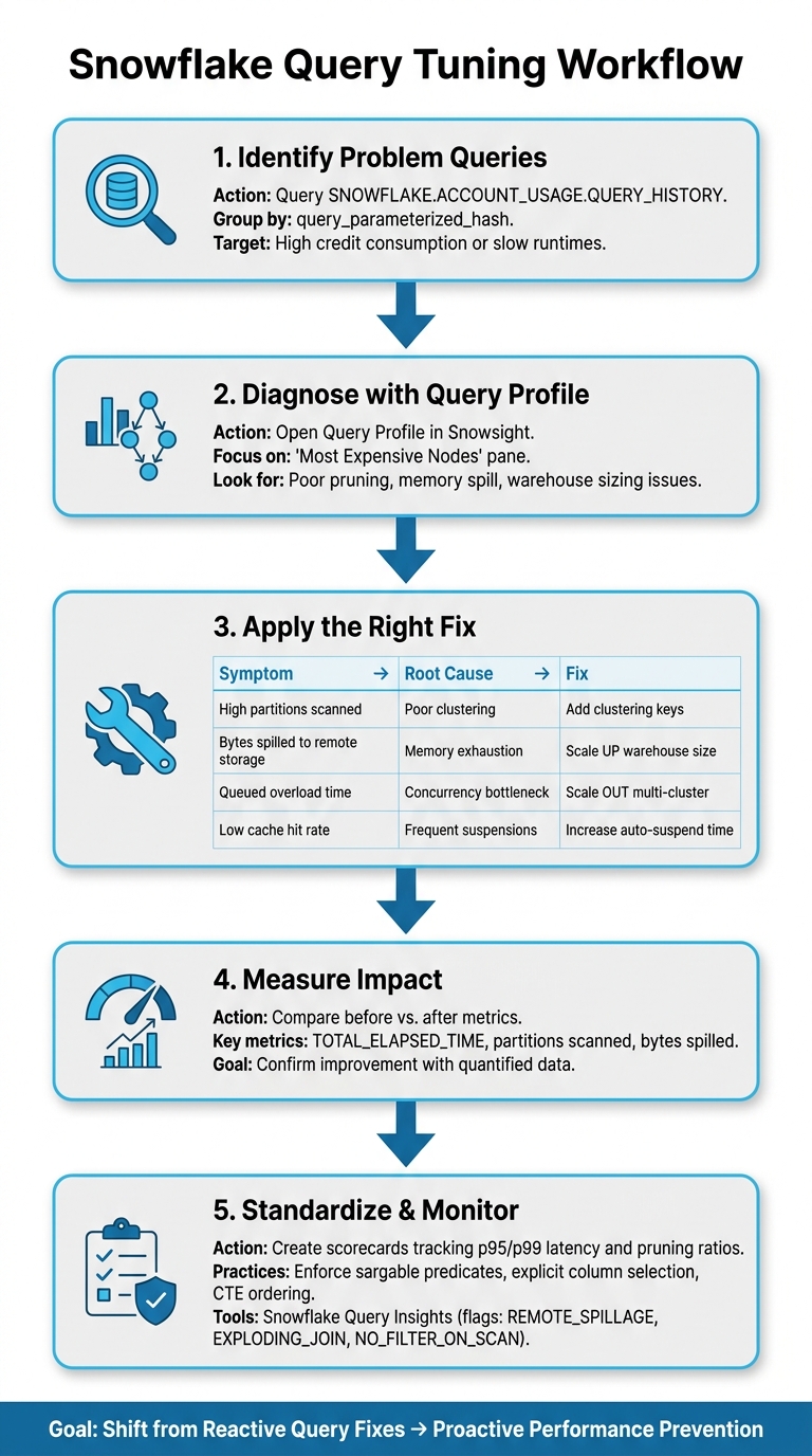
Snowflake Query Tuning Workflow: Step-by-Step Optimization Process
Optimizing individual queries can be helpful, but the real game-changer is turning those one-off fixes into a consistent strategy for long-term performance. A structured workflow ensures that improvements stick and deliver ongoing results.
A Step-by-Step Tuning Process
The first step is to identify the queries causing the most trouble. Dive into the SNOWFLAKE.ACCOUNT_USAGE.QUERY_HISTORY table and group by query_parameterized_hash. This will help you spot queries that are consuming excessive credits or running too slowly. These are your prime candidates for tuning.
Once you've zeroed in on a slow query, open the Query Profile and focus on the "Most Expensive Nodes." This step helps uncover issues like poor pruning or improper warehouse sizing. For example, scaling a warehouse from X-Small to Extra-Large has been shown to eliminate remote spilling, significantly cutting both runtime and cost.
"Snowflake is fast out of the box but not auto-magical... you don't need folklore…you need a method... we're gonna start treating performance as a product." - Yaniv Leven, Seemore Data
After implementing a fix, measure the impact by comparing metrics like TOTAL_ELAPSED_TIME and the number of partitions scanned. Over time, you can create scorecards to track pruning ratios and latency metrics (e.g., p95/p99) for your models or reports. This proactive approach helps catch performance issues early, before users notice.
With a solid process in place, the next step is to standardize these practices across your team.
Query Standards and Governance
Fixing performance issues is just the beginning. To ensure lasting improvements, it's essential to implement standardized coding practices that guide your team toward consistent results.
One key takeaway is that most performance gains come from early filtering and pruning, not just faster execution. This principle should shape the SQL standards your team adopts.
Some best practices include:
- Using sargable predicates to improve filtering.
- Selecting columns explicitly rather than using
SELECT *. - Maintaining consistent ordering of Common Table Expressions (CTEs).
For structuring queries, the dbt import pattern is highly effective. Organize CTEs in this order: Imports → Filtering/Cleaning → Aggregations → Joins → Final Projection. This setup helps Snowflake's optimizer follow a clear and predictable path. Additionally, use UNION ALL instead of UNION unless deduplication is absolutely necessary.
"Treat the optimizer as a partner. Write 'optimizer-friendly' queries that guide Snowflake to the best path." - Ronnie Joshua, Principal Data Engineer
Code reviews are critical for enforcing these standards. Queries that scan entire large tables without a WHERE clause should be treated as seriously as a security vulnerability - flag them, fix them, and document the changes. Snowflake's Query Insights tool can assist by automatically identifying anti-patterns like REMOTE_SPILLAGE, EXPLODING_JOIN, and NO_FILTER_ON_SCAN. These flags give reviewers a clear starting point for improvements.
Training and Skill Development
Establishing standards is important, but ongoing training ensures your team can maintain and expand on those improvements. Hands-on learning is particularly effective for understanding concepts like dynamic pruning, join build-side selection, and scaling strategies (both vertical and horizontal).
DataExpert.io Academy offers training programs tailored to these needs. Their boot camps and subscriptions focus on practical, real-world scenarios with Snowflake, including capstone projects and tools to build performance pattern recognition. Combining this kind of training with strong standards helps teams shift from reactive problem-solving to proactive performance management.
Conclusion: Steps to Low-Latency Performance in Snowflake
Achieving low latency in Snowflake involves a combination of compute, storage, and query optimizations. To start, focus on optimizing compute - right-sizing your warehouses is a quick win that can yield immediate results. Next, refine your storage strategies by leveraging clustering keys and Search Optimization. Finally, fine-tune your SQL queries by employing techniques like using sargable predicates, selecting only the columns you need, and stabilizing query text to maximize Result Cache hits. For instance, if more than 20% of partitions are being scanned in your queries, it’s a clear sign that pruning isn’t working effectively. At that point, revisiting clustering strategies or applying Search Optimization should be your next step.
"Warehouse tuning is about giving your queries the right engine. Storage optimization is about building better roads. You need both, but they address different problems."
By aligning strategies for compute, storage, and SQL, you can achieve consistently low latency. Here’s a quick summary of the key optimization levers and when to apply them:
| Optimization Lever | Target Bottleneck | When to Apply |
|---|---|---|
| Warehouse right-sizing | Memory spill / compute issues | First - quick to implement |
| Workload isolation | Queuing / concurrency | Early - to avoid resource competition |
| Clustering keys | Poor partition pruning on large tables | After compute is stable |
| Search Optimization | Point lookups on high-cardinality columns | For specific, targeted queries |
| Sargable predicates & column pruning | Excessive data scanned | Every query, every time |
| Result Cache stabilization | Repeated dashboard queries | Ongoing - low effort, high return |
This step-by-step approach not only focuses on technical fixes but also ensures smooth team execution. Building a skilled team is just as important as the tuning itself. Platforms like DataExpert.io Academy offer hands-on Snowflake training, equipping engineers to move from reactive query fixes to proactive performance optimization. The ultimate goal? A team that doesn’t just solve slow queries but prevents them from happening in the first place.
FAQs
How do I know if I should scale up or scale out my warehouse?
To figure out the best approach, start by identifying the type of bottleneck you're dealing with:
- Scale up: If your queries are slow due to heavy computation, large data scans, or memory limitations, consider increasing the size of your warehouse. You can test this by running the query on a larger warehouse - if it runs much faster, scaling up is likely the right choice.
- Scale out: If the issue is related to concurrency, such as queries getting queued, scaling out might be the solution. Adding more clusters allows the system to handle more simultaneous requests without impacting the speed of individual queries.
What’s the fastest way to spot why a query is slow in Snowsight?
To figure out why a query is running slowly in Snowsight, head to the Query Profile tab within the Query History. Pay close attention to the Most Expensive Nodes section, which highlights resource-heavy operations such as TableScan, Join, or Aggregate. Check the Query Insights for potential performance issues along with suggested solutions. Additionally, keep an eye on key metrics like Partitions Scanned vs. Total to assess pruning efficiency and Bytes Spilled to Remote Storage to spot memory-related bottlenecks.
When should I add a clustering key (and when is it not worth it)?
When working with large tables (over 1 TB) that are frequently queried but updated infrequently, adding a clustering key can make a noticeable difference. This is especially helpful when partition pruning starts to degrade or when the columns used in filters or joins differ from the table's ingestion order.
However, clustering keys aren't always the right choice. Avoid using them for:
- Small tables where the overhead isn't worth it.
- Tables that are updated frequently, as this can lead to inefficiencies.
- Queries that are already performing well without them.
Additionally, be cautious with clustering keys that include too many columns or columns with high cardinality. These can end up consuming extra credits without delivering meaningful performance improvements.